Randomness is seemingly all around us. Which popcorn kernel will pop next? How big will the next bubble in my lava lamp be? Where will the next raindrop hit me? Finding the answer to any of these questions is no better than a guess. All of these events are random by definition: their outcome cannot be easily guessed. It follows that if you record many instances of a possibly random occurrence, we would find no correlation, no patterns, and the results would be evenly spread over the possible space.
As it turns out, a lot of our perceived randomness truly is random. For sensitive applications, that is exactly what your computer uses. For instance, if you need to encrypt your hard drive, dedicated programs will use elements such as recorded environmental noise or mouse movement to generate random numbers that cannot be truly guessed. While this process is effective, it hardly is efficient; if you were to run a large-scale simulation where you’d need multiple draws of random numbers, recording it would take a while.
Digital systems can also generate random numbers, using deterministic processes. These programs are fast and efficient, but also deterministic and periodic. For all practical uses, their periods are usually long enough for it not to matter, but it still is a limitation. Given their determinism and dependence on initial conditions, algorithms used to generate random numbers are usually called pseudo-random number generators. Multiple different programs make use of pseudo-random number generators, from modeling and simulation suites to videogames.
Simplifying extremely, pseudo random number generators (PRNGs) have three main components: a generating process, an initial seed, and an extraction function. Why do you need a process? Consider generating a random number in, say, Julia: calling rand() will return a random floating-point number. If you call it again, you would like the resulting number to be different. And the one again after that. And the 1000th after that too; that is the whole point after all. So, the process that gave you the previous number has now to find a way to give you another one either different or not guessed better than random. Hence the problem: finding a deterministic function that can produce numbers that are statistically random from one draw to the next. The generating function might return a single float, an array of integers, or a matrix of complex numbers. How you transform the output of the generating function into a random number is the role of the extraction function. More on this later. Finally, the seed represents the initial conditions of the process. Usually the seed is passed to the generator as an integer. For instance, consider the following generator, the default in many programming languages: MersenneTwister(). The seed is usually passed to the generator like so rng = MersenneTwister(42) (you will find a lot of seed 42s around if you are on the lookout for them). Calling a random number with the generator and seed specified will now return the same number on my machine and yours rand(rng) = 0.7108238673434464.
One of the generating processes used in PRNGs I find most interesting is cellular automata (CA). If you were a researcher in the 80s, CA were all the rage; thanks to the increased availability of compute, simple computational processes provided a nice way to explore emergent behavior from simple rules. Taking a step back, CA are computational models composed of a grid of cells. Each of these cells can be in a certain state; for instance, the states can take values of 1 (indicating the given cell is active, alive, etc.) and 0 (inactive, dead, …). A given cell will evolve from time t to time t+1 according to its value and the value of the cells within a radius of it, i.e. its neighborhood. Finally, how the cell evolves is determined by a rule. Through these simple components, CA are able to model different patterns in multiple phenomena, and are subject to analysis themselves.
How can CA be used as generating processes for a random number generator? Let us focus on a simple case of cellular automata: one-dimensional grid, nearest neighbors (so, neighborhood radius of 1), and binary values for the cell’s state (0, 1). Stephen Wolfram studied these elementary CA (ECA) extensively, providing their nomenclature and classification. Specifically, one class of ECA seems to showcase chaotic behavior. Of the rules in the chaotic class, rule 30 also shows an additional interesting property: starting from a single active cell in the initial array, its central column shows no signs of periodicity or predictability. Given the potentially random properties of the central column of rule 30, Wolfram proposed a random number generator based on it. Allegedly, the PRNG of earlier versions of Mathematica did indeed use the central column of rule 30 as the generating process. When I was a master’s student reading Wolfram’s A New Kind of Science I got fascinated by the idea of creating random numbers from CA. However, I could not test it: I was lacking the programming skills, and frankly I had other priorities at the time. Now I have more priorities, and my computational skills haven’t gotten that much better; it seems like the right time to try my hand at it. I know Julia best, so I will be using it for the implementation. As luck would have it, I also already have a CellularAutomata.jl package implemented. What were the chances of that.
Now, the role of the seed in generating randomness from CA is relatively straightforward. If we let the chosen rule start from a single active cell, placed in the middle of the grid, we will always get identical evolution. We would then discard large numbers of initial generations (a transient) to obtain new states, making it dependent somehow on the seed value, ending up with a lot of wasted compute. It also would mean that the evolution of rule 30 (or any other rule) would essentially sit in the same trajectory. While historically accurate, that method does not make for a good PRNG. The chosen seed is therefore passed through a splitmix64 PRNG to generate (pseudo)random initial conditions dependent on the seed value. Am I cheating to hard-code a PRNG in a PRNG? Maybe. Of course, discarding an initial transient should always be allowed. Therefore, we will let our CellularAutomatonRNG have a warmup keyword.
Once we have defined the generating process and the seed, the only thing missing is transforming our information into randomness. If Wolfram is to be believed, the central column in rule 30 already is random! Treating each central cell in consecutive evolutions as 1 bit in a 64-bit integer, we define a new unsigned integer simply by letting the CA evolve and filling in the numbers. The process is pictured in Figure 1. If you want random booleans, then we will just set the cell value at face value: 0 or 1. Lastly, if we want floats, we take 53 bits, convert them into a big integer, and then divide by 2^53. The process should return floats in the [0, 1] range.
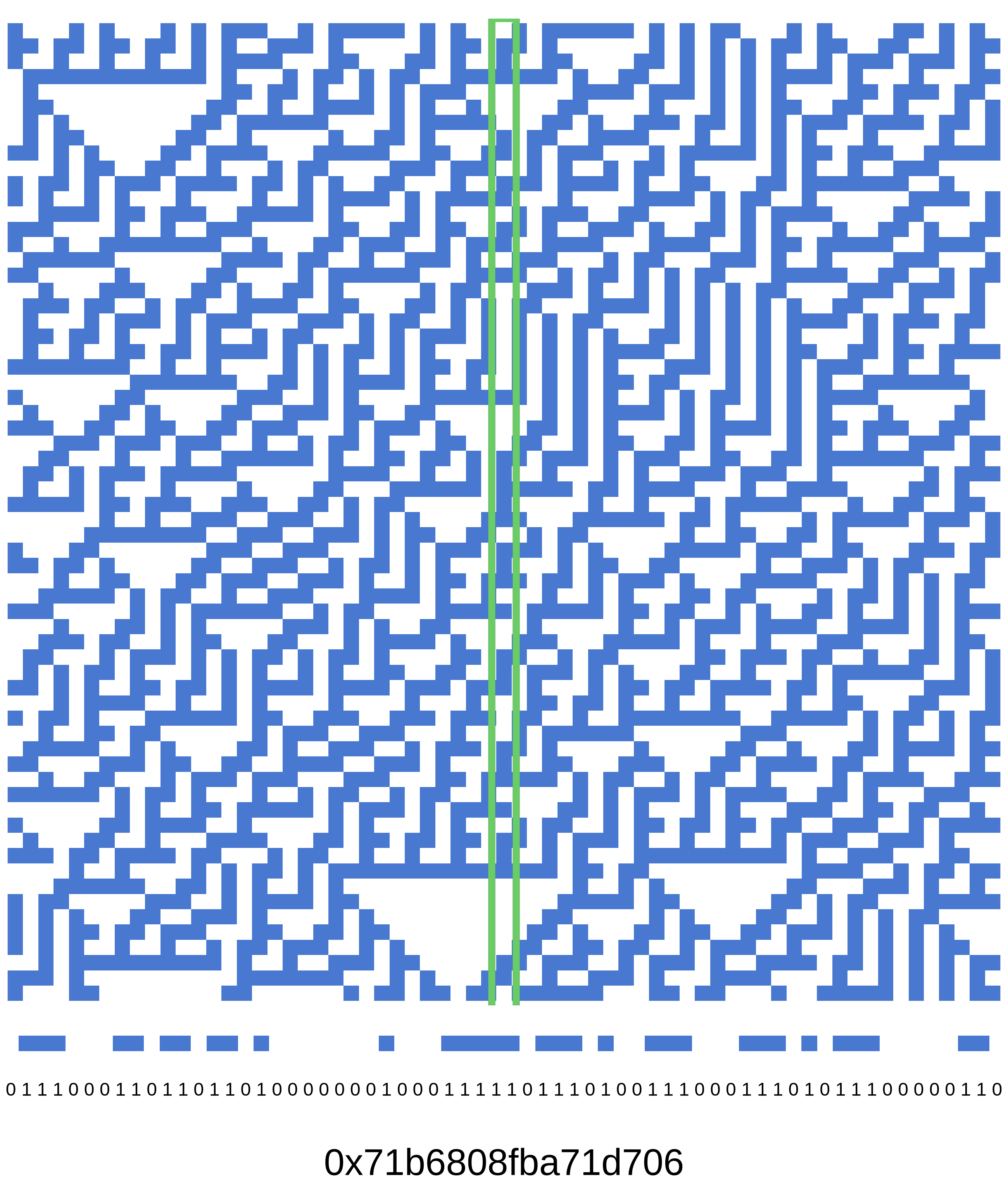
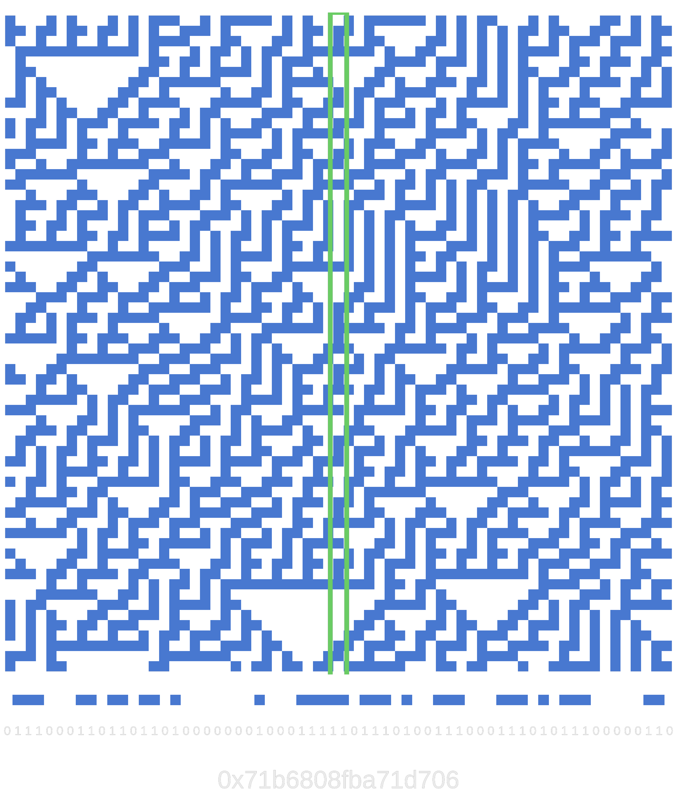
The astute and knowledgeable reader might notice that I pulled a slight trick; according to Wolfram, the central column is random when we start from a single active cell in the middle of the initial grid. However, we are starting from random initial conditions. Does that make a difference? I honestly do not know, but since I have implemented the generator in Julia, I can easily hook it up with the standard library’s Random machinery and generate some random numbers. The generated random numbers can then be fed into some RNG testers: these programs use some statistical approaches to determine whether a given sequence of numbers was generated by a process that could be random or not. dieharder is one of these tester programs, and the one I have used. The CellularAutomata.jl documentation showcases how random the numbers generated with rule 30 are. It does seem that the rule 30 central column cells maintain a good level of randomness, even if we are not starting from the single active cell.
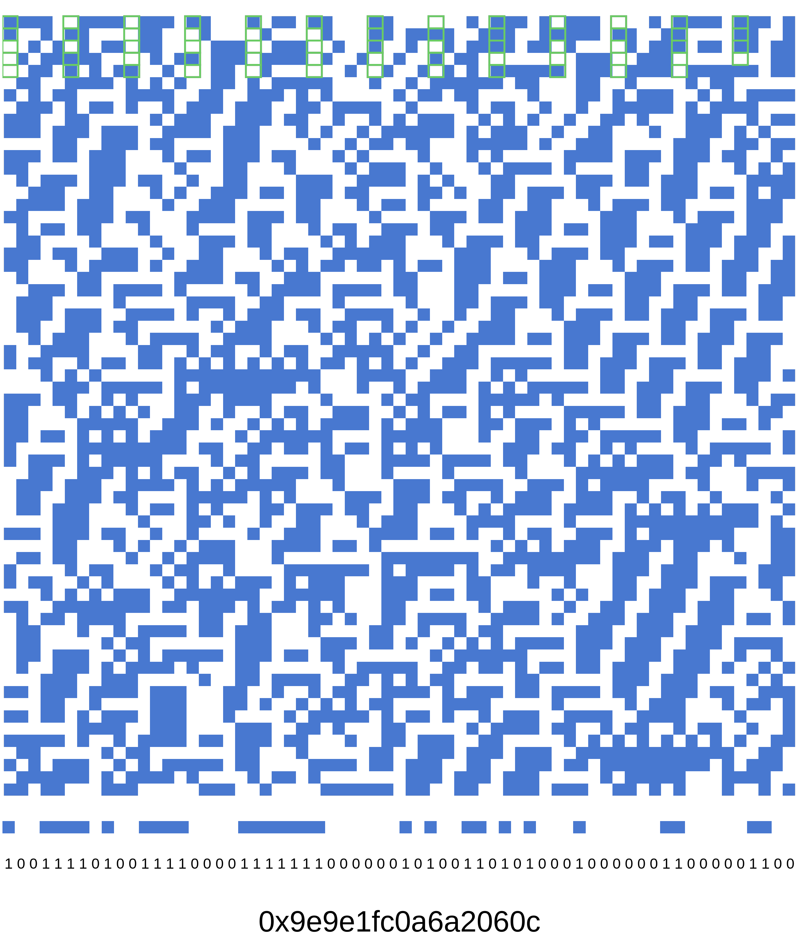
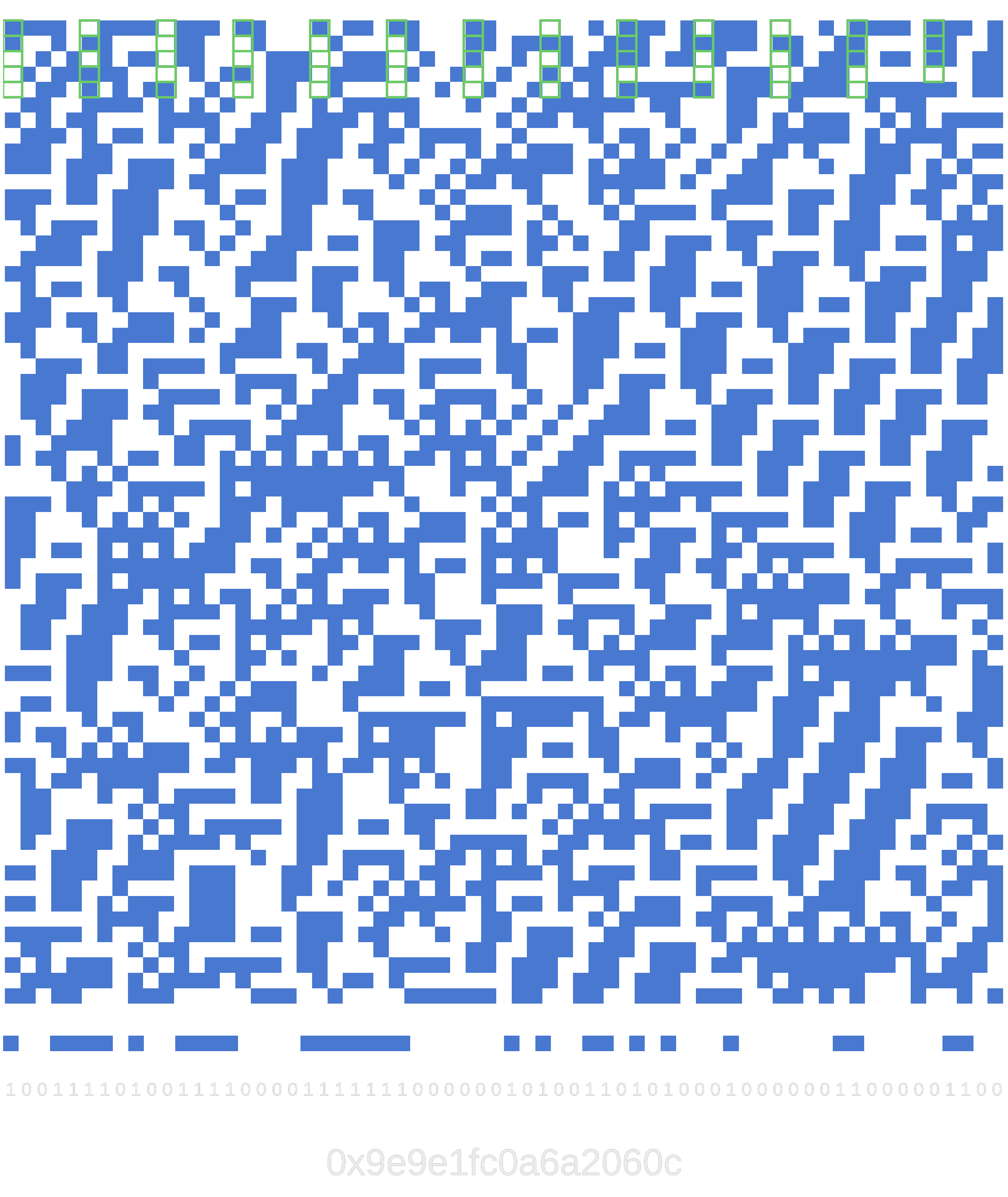
Nowadays, the default RNG in Mathematica is still based on CA, but not on rule 30. The new method is ExtendedCA, which is based on a CA with a larger neighborhood radius of 2. The larger radius means that each cell’s evolution now depends on the previous 5 values: its own its own value in the previous generation, plus the value of the four neighbors. The extension of the radius means that the evolution of the CA could provide more complicated patterns, carrying more potential for randomness. Additionally, the new approach does not use the central column only. From a given evolution of cells, it starts reading bits from index start; additional bits are read jumping from one cell to the next at distance skip. How random numbers are created from the CA bits is kept identical to before, as illustrated in Figure 2. The generating CA in Mathematica is no longer specified, so I cannot really provide the same CA to generate random numbers as they do. I tried to use a random looking CA, but the results were not statistically satisfactory.
Overall, creating a random number generator from cellular automata was a fun evening. Randomness is not my main field of expertise, so I have no say in the true randomness of the numbers generated with a CA. I do not think that you should use my own implementation for any serious cryptographic work, but I will sneak it in some of my academic simulations. If you want to explore it yourself, please head over to CellularAutomata.jl, install it, and give it a try:
using CellularAutomata
using Random

rng = CellularAutomatonRNG(DCA(30); size = 127, seed = 1)
rand(rng, Float64, 5, 5)
5×5 Matrix{Float64}:
 0.924718  0.0397089  0.650766   0.658859  0.478524
 0.249671  0.0518914  0.780269   0.465178  0.551268
 0.955349  0.0439952  0.0913971  0.361326  0.0310229
 0.737242  0.941889   0.726398   0.851282  0.499157
 0.236041  0.923313   0.871192   0.558179  0.976343